📦
Many target distributions
SplineGrid, PolynomialGrid, SumOfGaussians, Mesh, and more — all supporting smoothing for faster convergence
Fast · Differentiable · N-dimensional — works natively with JAX and PyTorch.
Here is a computation of the Wasserstein 2 distance between a sum of dirac and a spline grid:
from sdot import SplineGrid, SumOfDiracs, distance
import numpy as np

f = SumOfDiracs( np.random.rand( 1000, 2 ) ) # 1000 equal-weight diracs in 2D
g = SplineGrid( np.random.rand( 10, 10 ) )   # random 10×10 spline density, C0 by default (auto-normalized)

print( distance( f, g ) ) # by default, used the 2 norm as the ground metric
If not already loaded, SDOT automatically picks the best available backend (JAX, then PyTorch) and device. Configure it →
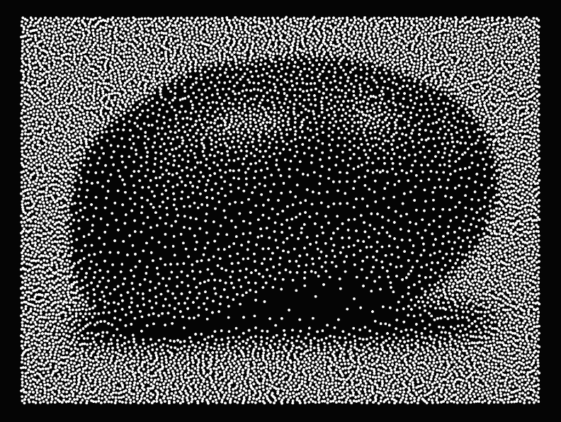
Given a discrete measure f (a weighted sum of Dirac masses) and a continuous density g, semi-discrete OT finds the power diagram (Laguerre tessellation) that partitions space so that the mass of each cell matches the weight of the corresponding Dirac.
The solution is unique, and can be computed via a provably-convergent Newton algorithm in O(n log n) time — making it practical for very large number of points in 2D, 3D or more, and can easily achieves machine precision if required.
Reference: Kitagawa, Mérigot, Thibert — Convergence of a Newton algorithm for semi-discrete optimal transport, JEMS 2019.
Of courses, sdot allows to access quantities of the transport plan.
from sdot import SplineGrid, SumOfDiracs, optimal_transport_plan
import numpy as np

f = np.random.random( [ 30, 2 ] ) * 2 - 1 # seen as dirac position
g = Box( frame = [ [ 0, 0 ], [ 2, 0 ], [ 2, 0 ] ] )

plan = optimal_transport_plan( f, g )

print( plan.barycenters ) # centroid of each transport cell
print( plan.cells )       # batch of cells, with possible access to vertices, edges, ... with gradient enabled
print( plan.second_order_moments ) # ...

plan.backward_map.brenier_potential.plot()  # the dual potential ψ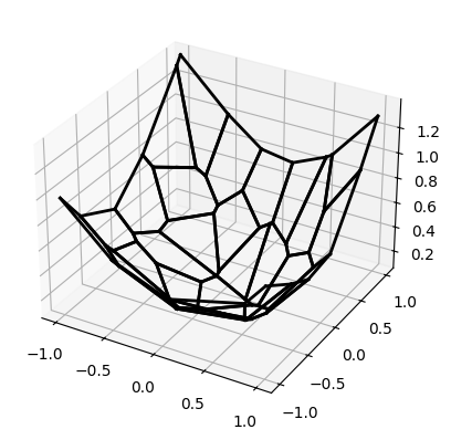
Virtually all the outputs can generated gradients. Here is an example with distance:
@jax.jit
def loss( positions ):
    f = SumOfGaussians( positions )
    g = SumOfDiracs( diracs )
    return distance( f, g )

diracs = np.random.normal( [ 1, 2 ], 0.3, size = ( 50, 2 ) )
grad = jax.grad( loss )( jnp.array( [ 0.0, 0.0 ] ) )
Of course, it applies on all the other quantities (e.g. barycenters, cell vertices) with respect to all input quantities (images values, ...).
SDOT has been used for:
See the Examples gallery →