Examples
The features of SDOT, each shown at work on a page of the guide, and use cases that put them together.
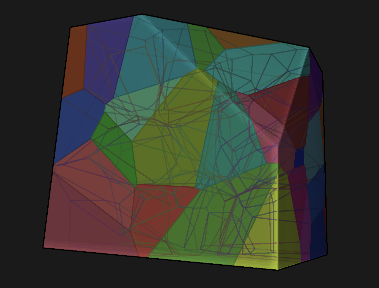
The Lebesgue measure on a convex polytope: a box, half-spaces, a convex hull, in 2D and 3D.
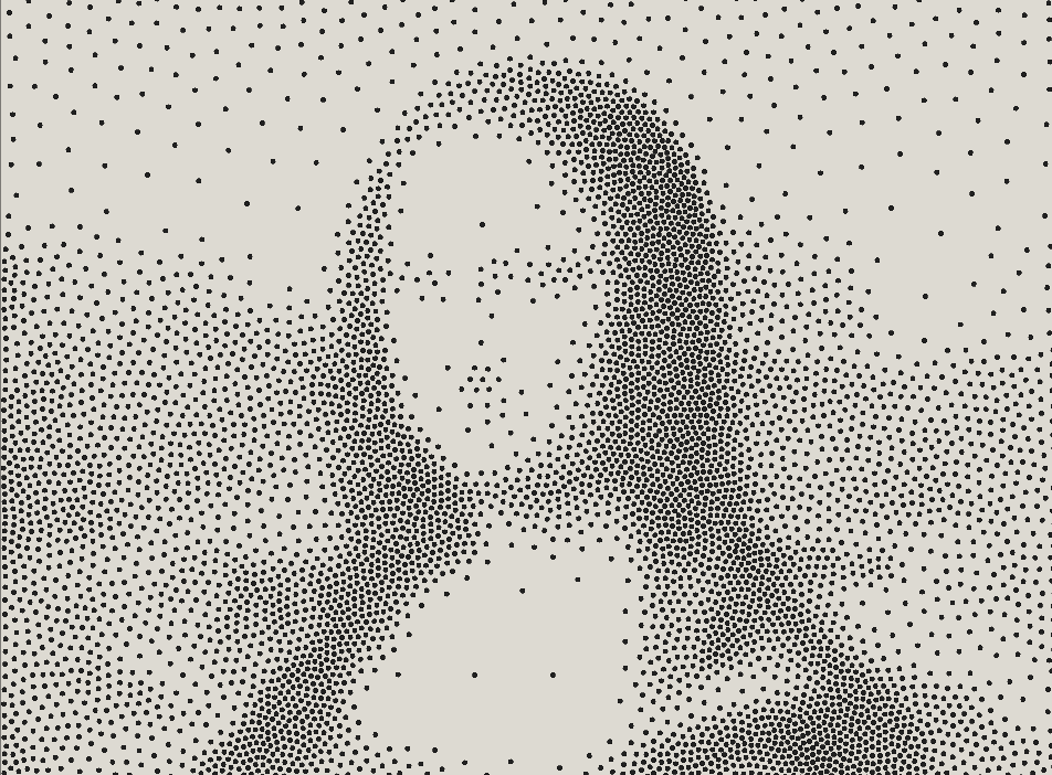
Piecewise constant or polynomial densities on a grid of pixels, and smooth B-splines.
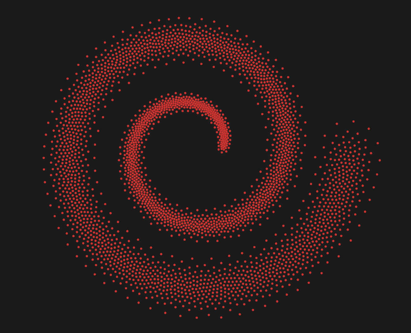
A mixture of isotropic gaussians as a continuous target.
Piecewise linear densities on triangles or tetrahedra: domains of any shape.
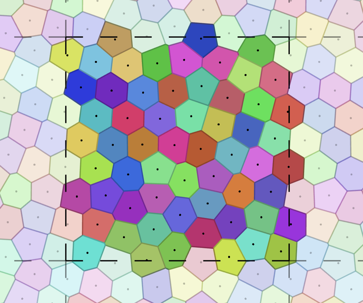
Targets carried by segments or triangles of lower dimension than the space.
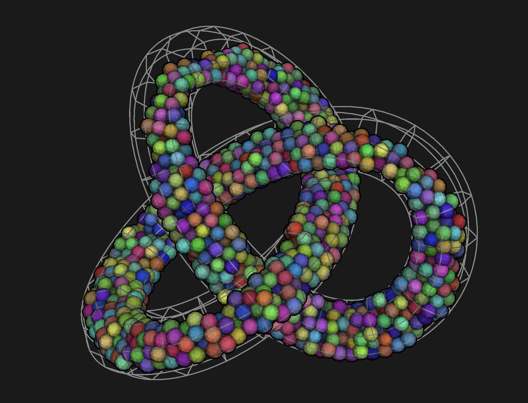
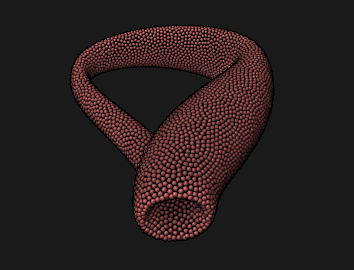
OT on quotient spaces — a torus, a Klein bottle, a cone... — from any group of isometries.
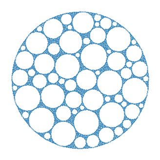
Clouds seen along lines: projected diracs, tents and domes, transported to one profile per direction.
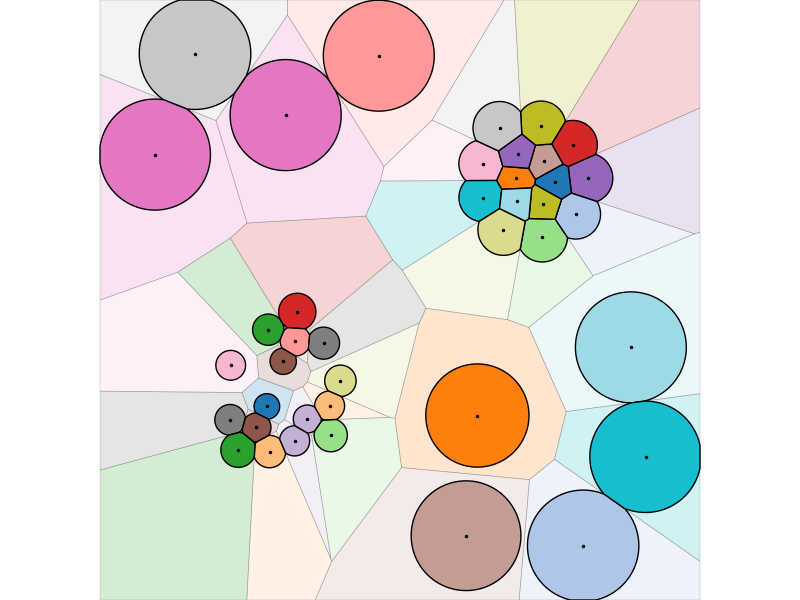
A source lighter than the target, the rest of the target going to a sink.
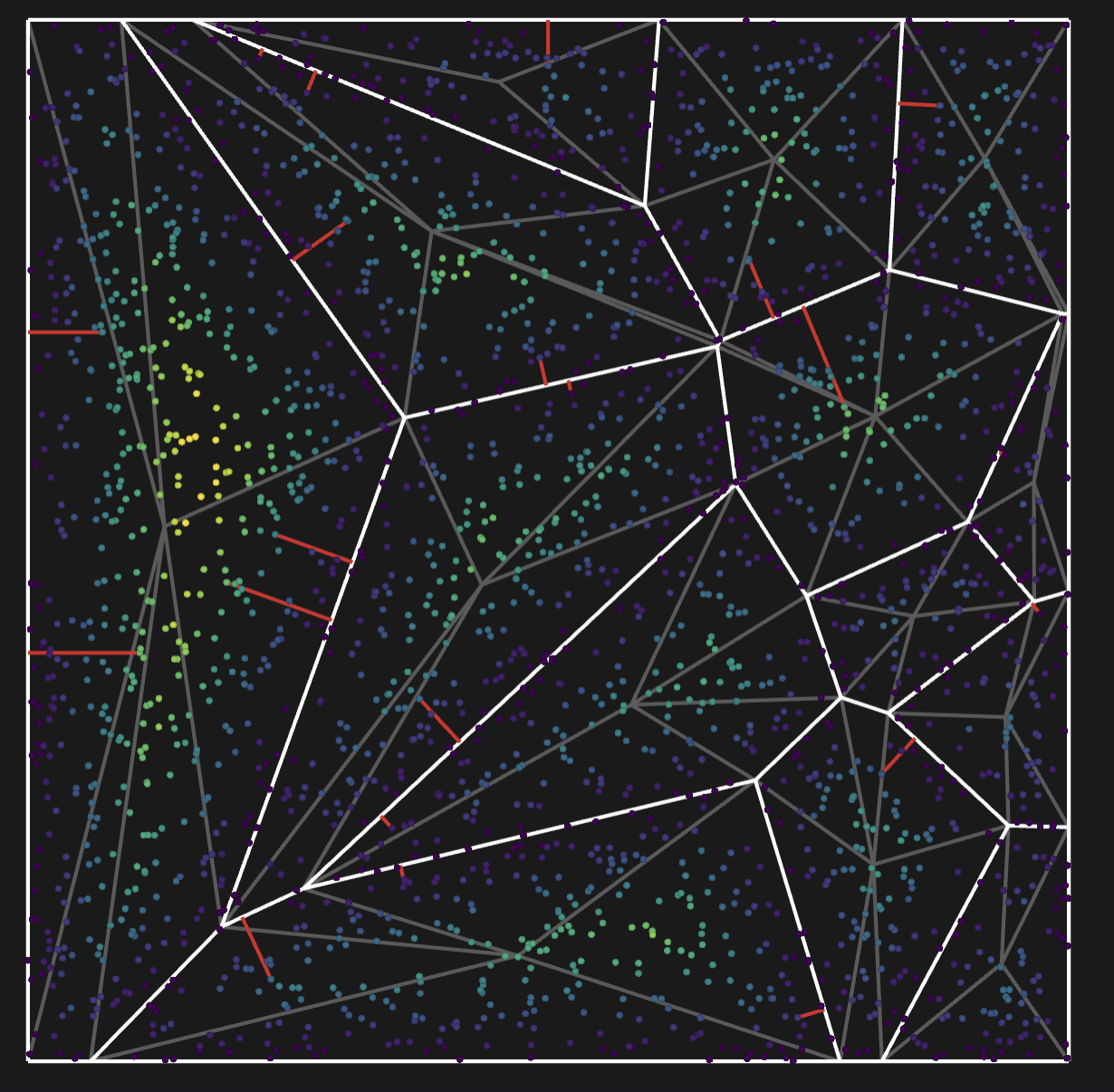
Walk the geometry of a power diagram: vertices, edges, facets and cells, each once, with their parents and children, simplices and distances — also on a torus.
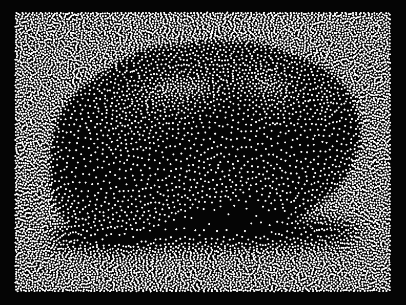
Iteratively move Diracs to their transport barycenters — converges to an optimal quantization of the target density.
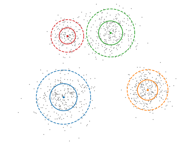
Fit the parameters of Gaussians to a point cloud by minimizing W2, by gradient descent then L-BFGS. Demonstrates the use of gradients.
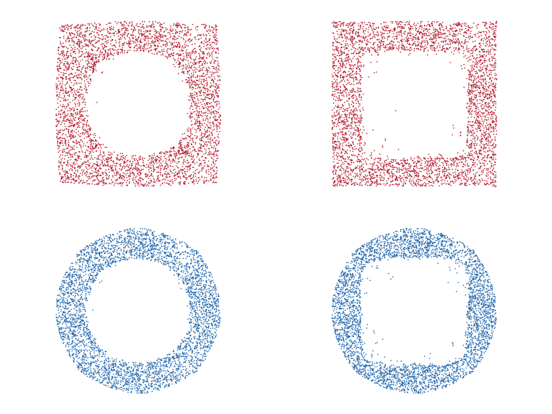
Embed point clouds by their transport map from the Lebesgue measure of the unit square, learn a family of shapes by PCA of these maps, and identify new draws by projection.
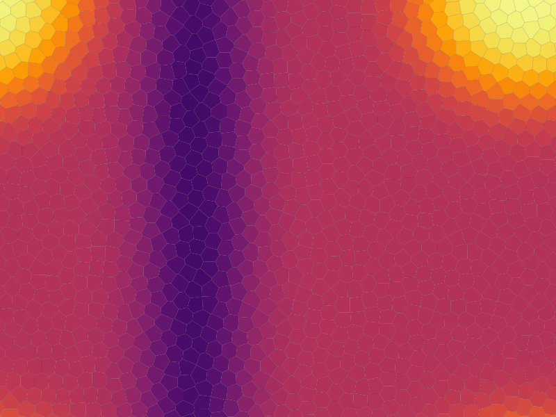
Finite volumes on power cells — the heat equation on a torus, from the facets of the cell complex.
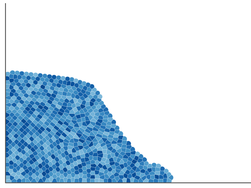
An incompressible fluid with a free surface, its particles being cells of a partial transport (Gallouët-Mérigot scheme).
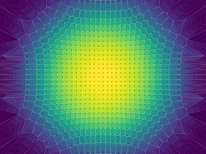
Linear diffusion with particles, the entropy being replaced by its Moreau-Yosida regularization (Leclerc-Mérigot-Santambrogio-Stra scheme).
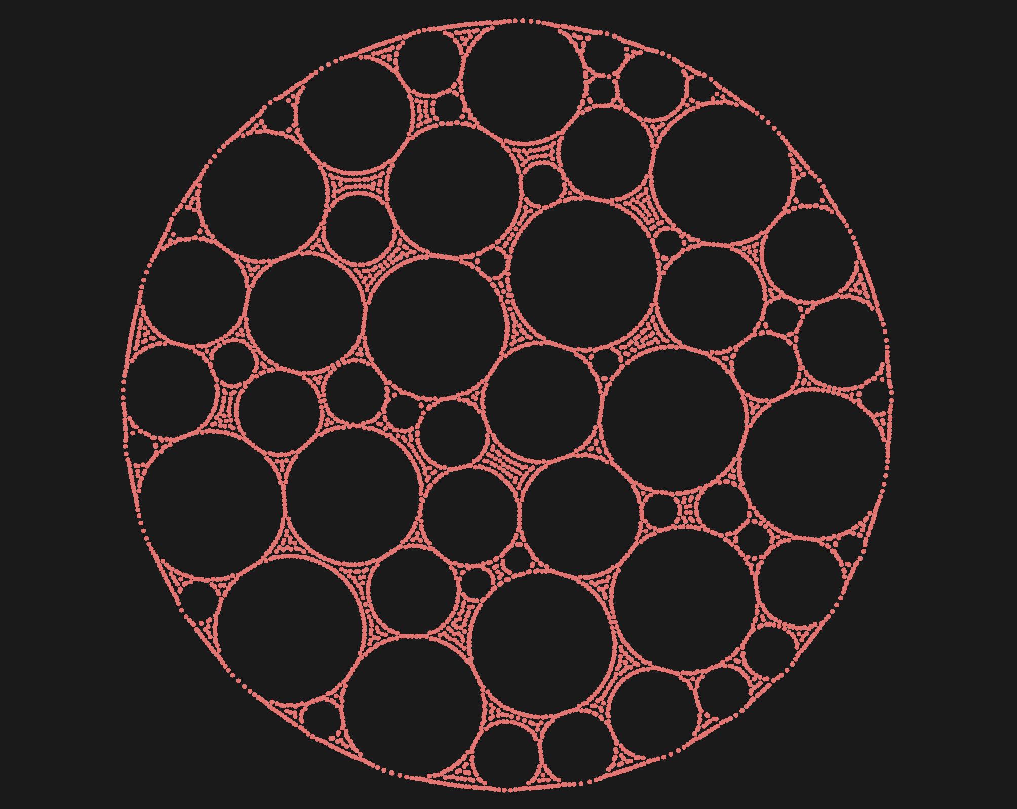
Reconstruct a density from its projections with a cloud of tents, coarse to fine, with L-BFGS — on a cylinder pierced by packed bubbles.