Skip to content

Fokker-Planck Diffusion ​

The Fokker-Planck equation ∂tρ=Δρ+div(ρ∇V) is the Wasserstein gradient flow of the free energy

E(ρ)=∫Vdρ+∫ρlog⁡ρ.

A Lagrangian discretization moves n particles xi of mass 1/n. The entropy of a sum of Diracs is +∞, so the scheme of L., Mérigot, Santambrogio and Stra (Lagrangian discretization of crowd motion and linear diffusion, SIAM J. Numer. Anal., 2020, arXiv:1905.08507) replaces it by its Moreau-Yosida regularization:

Hε(μ)=minσ12εW22(σ,μ)+∫σlog⁡σ.

The optimal σ is a power diagram whose cells carry a gaussian centered on their own particle:

σ(x)=e(ψi−|x−xi|2)/(2ε)on the Laguerre cell Li(ψ),where the weights ψ give ∫Liσ=1n for every i.

This is a semi-discrete transport where each cell integrates a radial function of its seed, radial_func = sdot.RadialExp( eps ). The gradient of Hε with respect to xi is (xi−bi)/(nε), where bi is the barycenter of σ on Li. The ODE x˙i=(bi−xi)/ε−∇V(xi) is integrated with explicit Euler steps.

python
problem = sdot.OtProblem( sdot.SumOfDiracs( x ), domain, radial_func = sdot.RadialExp( eps ) )
for step in range( nb_steps ):
    problem.source = sdot.SumOfDiracs( x )           # every cell gets the mass 1 / n
    b = np.asarray( problem.solve().barycenters )    # the barycenters of sigma
    x += tau * ( ( b - x ) / eps - grad_V( x ) )

With a radial function the masses no longer sum to a constant: raising every weight by c multiplies σ by ec/(2ε). There is no gauge to fix, and ∂mi/∂ψi has one more term, mi/(2ε), beyond the facets. The solver's Newton sees it as a sink of fixed weight: a ground node linked to each cell by that coefficient (sdotplan/Sweep.h). The start, the Voronoi diagram or the weights of the previous step, is raised so that σ weighs 1. The plan is differentiable, as any plan: positions, masses, values of the density. The cells and their integrals alone are sdot.PowerDiagram( x, psi, distribution = domain, radial_func = sdot.RadialExp( eps ) ).

Heat equation ​

V=0. The particles start on hZ2 inside the disk of radius 1/2, in the box [−1.5,1.5]2, with h=1/30 (one of the two discretizations of figure 6 of the paper), ε=8h2 and τ=ε/4. The color is σ, scaled by its maximum at each time.

Open in a separate page ↗

Inside the disk the cells are squares and σ is almost flat: the particles do not move. The cells on the edge of the disk reach the walls, and σ goes out along them, as far as ε from the particles. Their barycenters lie outside, which pulls the edge outward. Each particle then has room behind it, and the motion spreads inward.

The heat flow from a uniform disk is known: ρt=ρ0∗N(0,2t). Its second moment grows as r2/2+4t. On the left, the law of the distance to the center, particles against the exact flow; on the right, the second moment, for h=1/30 and h=1/80:
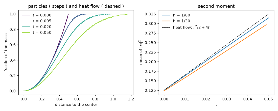
Particles against the exact heat flow

The choice of ε ​

ε is compared to the square of the spacing a of the particles. Two errors compete:

  • if ε is of the order of a2 or smaller, the gaussian of a cell is not flat over it, and the motion is slowed;
  • if ε is not small compared to the square of the scale of ρ, σ is a blurred version of ρ.

The slope of the second moment (4 for the heat flow) measures them. Between t=0.025 and t=0.05 (study in the script):

ε=2h2ε=4h2ε=8h2ε=16h2
h=1/30 (697 particles)3.393.563.603.48
h=1/50 (1941 particles)3.433.633.733.73
h=1/80 (5013 particles)3.663.783.83

The slope approaches 4 as h decreases: the gap is roughly proportional to h. The spacing that matters is the local one, which grows as ρ spreads: at ε=2h2 the slope drops over time (3.56 in the first fifth of the run, 3.39 at the end for h=1/30), while at ε=16h2 it rises (the blur fades as ρ widens).

The time step plays almost no part: τ=ε/10 and τ=ε give the same slopes as τ=ε/4. Each step takes about three Newton iterations ( to an absolute tolerance of 10−12 on the masses ), started from the weights of the previous step.

With a potential ​

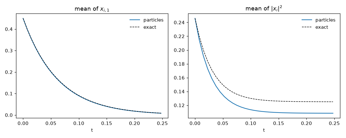
V(x)=|x|2/(2s2) with s=1/4: the equilibrium is the gaussian e−V, and the flow is that of an Ornstein-Uhlenbeck process, whose mean and second moment are known. The particles start on a disk of radius 0.3 centered at (0.45,0), with h=1/40, ε=8h2 and τ=ε/4.

Open in a separate page ↗

Mean and second moment against the Ornstein-Uhlenbeck process

The mean follows the exact decay e−t/s2. The second moment settles about 13 % below 2s2: the variance at equilibrium is proportional to the diffusion coefficient, and the diffusion is slowed as for the heat equation. At equilibrium the 437 particles are about 1/30 apart, as in the first row of the table above.

Limits ​

RadialExp works in 2D, with a density constant on pieces (Box, Image of degree 0, ConvexHull), on the CPU, without a periodicity or a sink. See the roadmap.

The pages are written by docs/examples/fokker_planck.py.

SDOT — H. Leclerc, Q. Mérigot, T. Gallouët · LMO / INRIA PARMA