Partial Transport

When the source weighs less than the target, only part of the target is transported, and the rest goes to a sink. The masses decide: each distribution is normalized to its target_mass ( 1 by default ).

p = sdot.plan( sdot.SumOfDiracs( positions, target_mass = 0.4 ), sdot.Box() )     # 40 % of the box is transported

Two equal target_mass values balance exactly; otherwise the masses are compared up to a relative ${10}^{-12}$. With target_mass = None, a distribution weighs what it holds: the sum of the weights of the diracs, or the integral of the density of an image. For instance, 30 diracs of uneven masses summing to $0.45$ against the unit square take $45\mathrm{\%}$ of it, a heavy dirac taking a bigger ball than a light one:

masses = rng.uniform( 0.2, 1, size = 30 ) ** 2
masses *= 0.45 / masses.sum()
p = sdot.plan( sdot.SumOfDiracs( positions, masses, target_mass = None ), sdot.Box() )

Open in a separate page ↗

What each dirac takes

The sink has weight $0$: a point $x$ goes to dirac $i$ when $|x-p_i{|}^2-w_i$ is the smallest power distance and is negative. In 1D, with three diracs ( weights chosen by hand ): each point goes to the lowest of the parabolas, or to the sink when they are all above $0$. The interval of a dirac stops either where another parabola gets lower ( a Laguerre facet ) or where its own parabola crosses $0$, at a distance $\sqrt{w_i}$ from it:

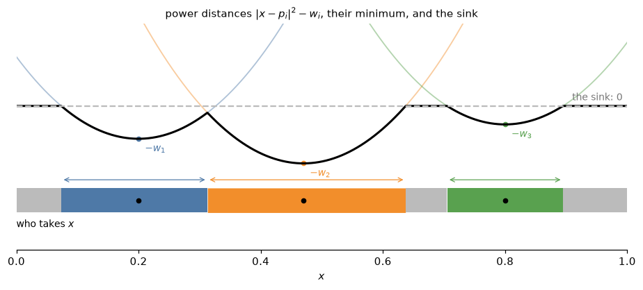
The cell of $i$ is its Laguerre cell intersected with the ball $B_i$ of radius $\sqrt{w_i}$, and the cost is $\sum _i{\int }_{L_i\cap B_i}|x-p_i{|}^2\rho$.

Visualization

The Laguerre cells are computed as usual. Only the integration is restricted to the balls, so add_to_viz draws the cells whole but faded ( opacity_beyond_balls ), with what each dirac transports in full color on top:

viz = sdot.Visualizer()
p.add_to_viz( viz )
viz.write_html( "partial.html" )

The mass of the source

40 diracs on a density in bands, the same positions, a source whose mass goes from 0.15 to 1 ( the slider at the top of the viewer ). At low mass the balls are disjoint, smaller where the density is high ( the same mass on a smaller area ). As the mass grows they meet, and the Laguerre facets split them; at a mass of 1 the transport is balanced, and the cells fill the square.

Open in a separate page ↗

Under the hood

The cells are not changed: they stay the Laguerre cells, and it is the integration that is restricted to the balls, in closed form ( a polygon inter a disc, for a density constant or affine on it: an Image, a Box, a Mesh ), with the derivatives. In 3D, a polyhedron inter a ball, for a density constant on it ( an Image, a Box, a Mesh( degree = 0 ) ): by the divergence theorem, the faces inter their discs ( the 2D closed form, in the plane of each face ) and the solid angles of the sphere inside the cell ( integration/InBall3.h ). For Newton, the sink is one more seed, whose target mass is what the diracs leave of the target and whose weight, $0$, is the gauge: the solver and its linear solvers are those of the balanced transport. The diagram takes it as PowerDiagram( ..., sink_weight = 0 ).

What is not supported yet

• a source heavier than the target ( an explicit error ), and the penalized variant ( a sink of fixed weight );
• targets that are neither constant nor affine on pieces ( SumOfGaussians, a polynomial Image ), and in 3D the affine ones too ( a Mesh of degree 1: Mesh( degree = 0 ) is constant on each tetrahedron ); the CUDA solve of an Image that is not a constant, the "limits" step.

On a GPU

The solve runs on a CUDA device in 2D for a constant density ( a Box, a Polytope ) or a Mesh, with or without a group of translations: the cells are integrated in their balls on the card, and the linear systems, bordered by the sink, are solved on the host ( the CPU's solver, on a copy of the laplacian at each iteration ).

The figures are written by docs/guide/ground-metrics/partial_figures.py.