Duplicates and Close Seeds

Two diracs at the same position have no plane between them: the power diagram is degenerate there, and so is everything computed on it. The cells overlap, the measures count the same region twice, the laplacian is singular, and the derivatives are meaningless. Two diracs 1e-9 apart do have a plane between them, but the doubles place it only to $\mathrm{ulp}(w)/(2\delta )$: no weight vector gives their cells the right masses to better than about 1e-6.

SDOT handles both with one convention. The seeds that are much closer to one another than to the rest form an aggregate. The aggregate shares one cell, which its members split among themselves, and it is written at its own scale, so that its planes are as precise as its positions. Aggregates nest: a pair 1e-12 apart inside a pair 1e-5 apart is an aggregate in an aggregate. This page explains the convention in the power diagram alone, then in the transport solver.

In a power diagram: a tree of aggregates

import numpy as np
import sdot

rng = np.random.default_rng( 0 )
positions = rng.random( ( 50, 2 ) )
positions[ 1 ] = positions[ 0 ]                          # an exact duplicate
positions[ 3 ] = positions[ 2 ] + 1e-9                   # a pair closer than the doubles can separate

pd = sdot.PowerDiagram( positions, boundaries = sdot.box_half_spaces( [ 0, 0 ], [ 1, 1 ] ), groups = "auto" )
print( pd.groups.members() )                             # { 0: [ 0, 1 ], 2: [ 2, 3 ], ... }
m = pd.measures                                          # every member has a cell of its own, the cells tile the box

Each aggregate in its own frame

An aggregate $A$ has a centre $b_A$ ( the barycentre of its diracs ) and a scale $D_A$ ( its size ). In its frame, $y=(x-b_A)/D_A$, each child ( a seed, or an aggregate nested in it ) has a virtual position and a virtual weight:

$$q=\frac{p-b_A}{D_A},W=W_A+D_A^{2}v.$$

Since $|x-p{|}^2=D_A^2|y-q{|}^2$, the power diagram of the $(q,v)$ in the frame of $A$ is exactly the true diagram, written where everything is of order one: the positions, the weights and the planes. The planes are placed as follows:

between	the plane	computed
a member and a seed outside its root aggregate	the ordinary power bisector	the true positions, and the outer weights $W$
two members of an aggregate	their true bisector	in the frame of their lowest common aggregate, from their virtual positions and weights there ( the deeper levels add $(D_{\text{child}}/D_A{)}^2$ times their own )
two exact duplicates	the bisector of their virtual diracs	unit directions $u_i$ around an apex, and their virtual weights

Seen from outside, an aggregate therefore behaves exactly like its seeds with their outer weights: its members tile its cell. Inside, each plane is computed at the scale of the two seeds it separates, at any depth. The outer weights are rounded, but only where the doubles could not have placed the plane anyway: far from the aggregate, it is a point.

Why virtual diracs for duplicates: the convention is a limit

Take two diracs $p\pm \delta u$ and let $\delta \to 0$. Their bisector passes through $p$, perpendicular to $u$, and shifts by the weight gap divided by $\delta$. In the limit, the cell of $p$ is split by the power diagram of seeds placed along $u$. Two exact duplicates whose virtual diracs are $p\pm ru$ get that limit split, whatever $r$ is: only the shape of the configuration matters, and the weights rescale with it. An aggregate of exact duplicates is the frame of scale $r$ where they sit at their unit directions; its virtual weights only split the cell of its site, they do not move it.

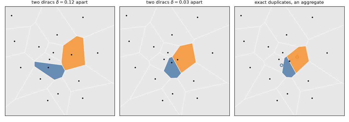
Left and middle: two diracs $\delta$ apart, in an ordinary diagram. Right: the same two diracs at the same position, an aggregate. The circles are their virtual diracs, and their split is the limit of the other two.

The weights given to the duplicates are then their virtual weights: they move the split inside the shared cell, as the weights of a power diagram do. groups = "auto" spreads the $k$ duplicates of a site in directions fixed by their rank: the regular polygon in 2D, deterministic springs on the sphere beyond. With equal weights their power diagram is a fan around the apex, so every duplicate gets a piece. The apex is the site, or, when the aggregate of duplicates sits inside a larger one, the site pushed a quarter of the local spacing away from the other children, into its own part.

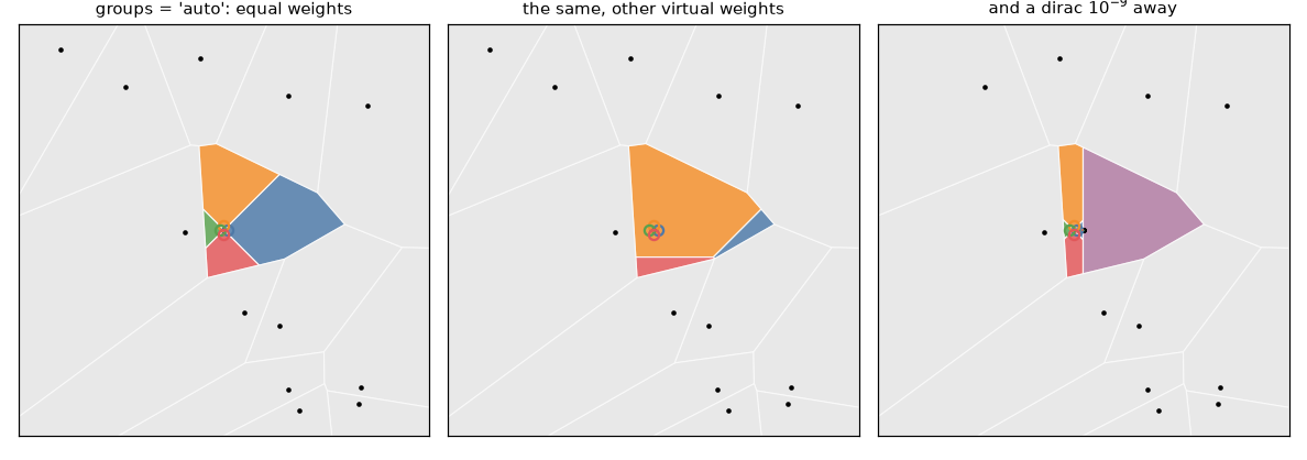
Left: four duplicates with equal weights, a fan. Middle: the same four with other weights, a different split of the same cell. Right: a fifth dirac 1e-9 away: the four duplicates become an aggregate inside the aggregate of the five, whose plane is computed at the scale 1e-9.

Which seeds are aggregated

groups = "auto" ( sdot.groups.find_groups ) reads the distances only: no weight, no tolerance, no gauge. It builds the single-linkage tree of the positions ( the dendrogram of their minimum spanning tree ). Each node of that tree is a set of diracs with a linkage height $d$ ( the longest edge inside it ) and the height $d_{\text{parent}}$ at which it joins the rest. The node is an aggregate when

$$d\le \kappa d_{\text{parent}},\kappa ={10}^{-3}\text{ by default }(\mathtt{\text{Tuning( aggregation\_kappa = ... )}}).$$

It is a separation of scales: seen from outside, the aggregate is a point. The criterion is recursive by construction, and the exact duplicates are the nodes of height 0. An ordinary cloud has no aggregate: its heights grow slowly, and in a uniform cloud of ${10}^5$ points the closest pair is near $h/300$. The computation is vectorized and done once: the exact duplicates by a hash of the positions, then the near neighbours of the distinct positions ( a k-d tree ), whose edges are merged by Kruskal in batches of lengths within a factor 2 ( a node and its parent in one batch are never $1/\kappa$ apart ).

An aggregate is never wrong: its planes are the true ones, so an extra aggregate costs a little work, never precision. The tree can also be given explicitly, as nested index lists ( groups = [ [ 0, 1 ], [ 2, [ 3, 4 ] ] ] ) or a sdot.Groups ( Groups.nested, Groups.from_rep for one level ).

Derivatives

measures and moment( k ) are differentiable with respect to the positions, the weights and the density, like those of any diagram. The planes of distinct positions are true bisectors, derived as such; the fans of duplicates follow their site. One case is a convention rather than a derivative. Move a single duplicate and the cells around it see its site through planes that coincide, so they are not differentiable. Their share is then the mean of the one-sided derivatives, which is what a centred difference sees. A site moved as a whole is differentiated exactly.

In the solver: every member its own mass

import numpy as np
import sdot

rng = np.random.default_rng( 0 )
positions = rng.random( ( 50, 2 ) )
positions[ 1 ] = positions[ 0 ]                          # an exact duplicate

plan = sdot.OtProblem( sdot.SumOfDiracs( positions ), sdot.Box() ).solve( sdot.Iterative( duplicates = "split" ) )   # the default
print( plan.groups.members() )                           # the groups of the plan
print( plan.stats[ "residual_full" ] )                   # each member's own mass, to the precision of the cells
b = plan.barycenters                                     # each member's own piece: 0 and 1 no longer share a barycentre

The tree is found before the first diagram, and Newton runs on all the weights of that geometry, with one unknown per seed ( the smallest seed of a node holds the unknown of the topmost node it is the smallest seed of ):

the slot	its unknown
a lone seed, or the smallest seed of a root aggregate	its outer weight $W$
the smallest seed of a child that is not the first of its aggregate	the child's virtual weight $v$, in its parent's frame

The first child of each aggregate is its gauge ( $v=0$ ). The jacobian is block triangular by levels, and a Newton step follows it ( sdotplan/Groups.h ):

1. The roots. Summed over a root aggregate, the masses do not see the planes inside it, so the rows and columns of each root are summed. The heavy coefficients of a close pair ( in $1/\delta$ ) cancel there. What is left is the laplacian of the roots, well conditioned, solved by the linear solvers of the transport ( the members are linked to their root, so the system keeps the size, the order and the gauge of the seeds ).
2. The aggregates, level by level. One small dense system per aggregate gives its children their virtual weights, from the sums of their masses. It is written in the aggregate's frame, at scale one: well conditioned at any depth.
3. The coupling back. A child's virtual weight also moves the outer weights, by $D^{2}v$: a coupling of relative size $(D_{\text{child}}/D_{\text{parent}}{)}^2\lesssim {\kappa }^2$. A few sweeps of block Gauss-Seidel on the residual handle it. None is needed when the tree only holds exact duplicates: their virtual weights do not move the cell of their site.

Every member's mass is tested, so the solve stops at the tolerance for each of them. The tree stays fixed during the whole solve: no criterion reads the weights, so no pair can turn up closer than expected.

A cloud without aggregates takes the ordinary path, unchanged to the bit. The card's solver ( 2D and 3D ) runs the same Newton: the cells of the members are made by a pass of their own ( one warp each, their planes in double in the seed's frame ), the roots' system is assembled and solved on the card, and the small blocks of the aggregates on the host. A periodicity and step = "limits" ( the 2D limits of the step do not know the groups ) keep the aggregation, which merges what the doubles cannot separate; each cluster then becomes a root aggregate ( with the separations of scales inside it as nested ones ), split by a Newton on its virtual weights. On the degenerate clouds of the tests, stats[ "residual_full" ] drops from about 1e-6 ( relative, for a pair 1e-9 apart ) to the tolerance on every path, the nested pair included.

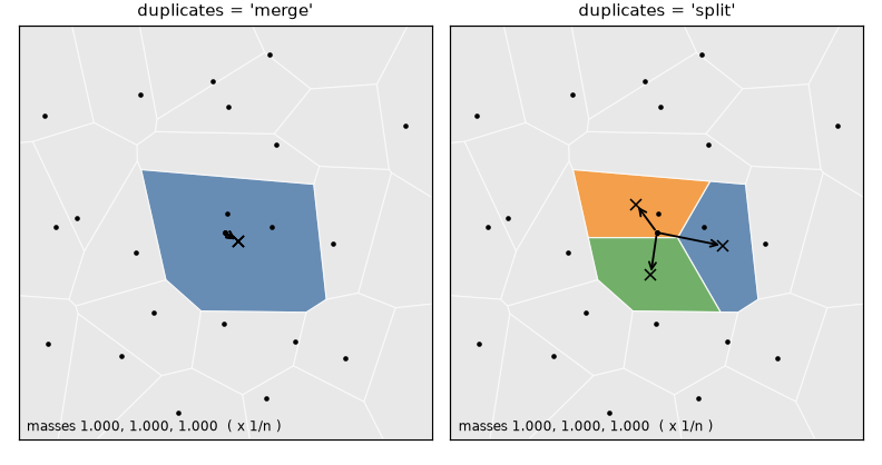
Three duplicates at the centre. Left, duplicates = "merge": they share the merged cell and its barycentre (×). Right, "split": a piece each, of its own mass, and its own barycentre. The arrows point from the diracs to the barycentres, the direction in which a descent moves them.

Why split: duplicates must be able to separate

The transport cost is semi-concave in the positions, and a duplicate sits on a concave crease. Every split of the shared cell among the duplicates is an optimal coupling, so the superdifferential of the cost there is the set of $2m_i(p_i-b_i)$ over all the splits. "merge" takes its centre, the fractional coupling: every duplicate gets the same gradient, so they move together and stay duplicates forever. "split" takes an extreme point, a split, which is the steepest descent. The duplicates get different gradients, and a descent separates them.

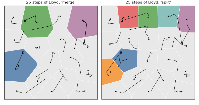
25 iterations of Lloyd ( each dirac to the barycentre of its cell ), from a cloud with three pairs of duplicates ( the squares ). With "merge", each pair stays one dirac in a cell twice too big. With "split", the pairs separate at the first step, and the six diracs settle like the others.

Derivatives of a plan with aggregates

Under jax.grad ( or any traced input ), the derivative of the plan comes from the implicit function theorem, level by level, as Newton solved it: one Newton step with the jacobian frozen, on the residual of the live diagram.

• the roots: PowerDiagram.laplacian_solve of the grouped diagram, the laplacian of the roots ( on the card, the card's: the members' cells by their own pass, the facets onto the roots );
• the aggregates, a level at a time: each one's dense block frozen ( its structure read from the tree, its values gathered from the facets on the backend: the same under jax.jit ). The directions of the duplicates are frozen too: the derivative is the one along the chosen split. So is the radius of their fan, which follows the spacing of the neighbours: the split does not depend on it, but the weight given to an exact duplicate past the first, $W+r^{2}v$, does, and its derivative leaves that dependence out.

The cost's gradient is the envelope one, member by member: $2m_i(p_i-b_i)$, with $b_i$ the barycentre of the member's own piece. The cost is written as the dual functional of the sites ( the distinct positions ) plus each member's offset from its site, so that this holds exactly, even for one duplicate moved alone; its weights' terms are written on the precise unknowns, each root's residuals summed first. For a pair 1e-9 apart, the true derivative is in $1/\delta$. It is exact, but it amplifies the rounding of the masses: about $\epsilon /\delta$ on the gradient.

duplicates = "merge" keeps the other convention: the outputs share the merged cell ( cell_masses in proportion to the masses, the merged barycentre for every member ), and the derivatives are those of one merged dirac.

Limits

• The aggregates are found on readable positions only. Under jax.jit they are not looked for ( give a Groups ), and a duplicate is then degenerate, as before.
• There are no groups with a periodicity yet. On the card, the dedicated cells take them in the solve and in laplacian_solve: a grouped PowerDiagram's other calls take the generic kernels.