Lloyd Quantization

An optimal quantization of a density $\rho$ is a set of $n$ Diracs $\mu =\frac{1}{n}\sum _i{\delta }_{x_i}$ that is as close as possible to $\rho$ in the Wasserstein sense:

$$\underset{x_1,\dots ,x_n}{min}{W}_2^2(\frac{1}{n}\sum _i{\delta }_{x_i},\rho ).$$

For fixed positions, the transport from the Diracs to $\rho$ splits the domain into power cells $L_i$ of mass $1/n$ each. The gradient of $W_2^2$ with respect to $x_i$ is $\frac{2}{n}(x_i-b_i)$, where $b_i$ is the barycenter of $L_i$ — so the fixed point is reached when every Dirac sits at the barycenter of its own cell. Lloyd's algorithm simply iterates

$$x_i\leftarrow b_i(x),$$

which decreases $W_2^2$ at each step. With equal masses, the result is a blue noise sampling of $\rho$: points as regular as possible, with a local density that follows $\rho$ (de Goes et al., Blue noise through optimal transport, 2012).

sdot.quantization

x = sdot.quantization( target, 1000 )   # 1000 Diracs, starting uniformly at random in the support
x = sdot.quantization( target, x0 )     # or from given positions

• target: any distribution (ConvexHull, SumOfGaussians, Image, ...);
• the starting point: either a number of Diracs, drawn uniformly at random in the support of target (seed makes the draw reproducible), or the positions themselves, [ n, d ], in any framework (NumPy, JAX, PyTorch, CuPy) — the result comes back in the same one;
• masses (optional): the mass of each Dirac, kept during the iterations — equal by default;
• periodicity (optional): Lloyd on a quotient space, a torus, a Klein bottle... (see Periodicity). The returned positions stay next to where they started, possibly outside the support;
• target_mass (optional): the share of target that the Diracs take, as a partial transport — 1 by default;
• radial_func (optional): a radial integrand around each Dirac, as in OtProblem (for instance sdot.RadialExp( eps )).

The iterations stop when the root mean square move of the Diracs is below tol times $\sqrt{W_2^2}$, i.e. the typical size of a cell. The default, tol = 2e-2, means the Diracs move by less than a fiftieth of a cell: the eye no longer sees anything. It takes about 20 iterations on the examples below; halving tol roughly doubles that. max_iter (200 by default) bounds the number of iterations.

Each iteration re-solves a transport, but the problem is kept between iterations: the previous weights are a very good starting point, and only a few Newton steps are needed.

To follow the iterations, pass a callback( iteration, positions, plan ). This is how the animations below were recorded:

history = []
x = sdot.quantization( target, 1000, callback = lambda it, pos, plan: history.append( pos ) )

Uniform density on a pentagon

1000 Diracs, starting uniformly at random in the pentagon.

import numpy as np
import sdot

angles = np.pi / 2 + 2 * np.pi * np.arange( 5 ) / 5
target = sdot.ConvexHull( np.stack( [ np.cos( angles ), np.sin( angles ) ], axis = 1 ) )

x = sdot.quantization( target, 1000, seed = 0 )

Open in a separate page ↗

Use the slider at the top of the viewer (or the play button) to go through the iterations.

A sum of three Gaussians

In 2D

2000 Diracs. support_sigmas = 3 truncates each Gaussian at three standard deviations: this is the domain of the transport.

centers = np.array( [ [ -0.5, -0.3 ], [ 0.5, -0.2 ], [ 0.0, 0.5 ] ] )
target = sdot.SumOfGaussians( centers, sigmas = np.array( [ 0.25, 0.15, 0.2 ] ),
                              weights = np.array( [ 1.0, 0.6, 0.8 ] ), support_sigmas = 3 )

x = sdot.quantization( target, 2000, seed = 0 )

Open in a separate page ↗

In 3D

Nothing changes but the dimension of the centers: 4000 Diracs.

centers = np.array( [ [ -0.5, -0.3, -0.2 ], [ 0.5, -0.2, 0.1 ], [ 0.0, 0.5, 0.3 ] ] )
target = sdot.SumOfGaussians( centers, sigmas = np.array( [ 0.25, 0.15, 0.2 ] ),
                              weights = np.array( [ 1.0, 0.6, 0.8 ] ), support_sigmas = 3 )

x = sdot.quantization( target, 4000, seed = 0 )

Open in a separate page ↗

An image

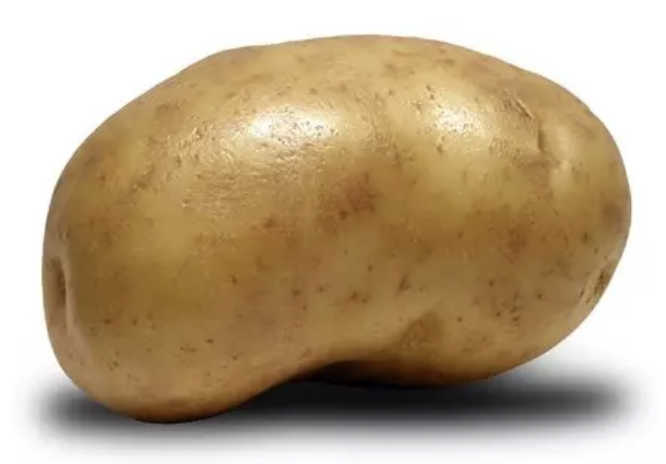
The density is now a piecewise constant image: the brightness of a photo of a potato — the white background is dense, the potato lighter, its shadow almost empty. 4000 Diracs, starting from white noise.

from PIL import Image

img = Image.open( "potato.png" ).convert( "RGBA" )
img = Image.alpha_composite( Image.new( "RGBA", img.size, "white" ), img ).convert( "L" )
img = img.resize( ( img.width // 4, img.height // 4 ), Image.Resampling.LANCZOS )

# sdot.Image indexes the pixels as [ x, y ], y upwards; + 1 keeps the density positive everywhere
values = np.ascontiguousarray( np.asarray( img, dtype = float ).T[ :, ::-1 ] ) + 1.0
target = sdot.Image( values )

x = sdot.quantization( target, 4000, seed = 0 )

Open in a separate page ↗

On a surface

The target can also be carried by a surface in 3D ( or by lines ): sdot.Mesh( nodes, triangles ), here a Klein bottle that crosses itself. The diracs start on the surface; see Lines and Surfaces for the details and the script.

target = sdot.Mesh( nodes, triangles )                  # 2880 triangles in 3D
x = sdot.quantization( target, 6000, seed = 0 )

Open in a separate page ↗

Reproducing the pages

The first four viewers above are written by docs/examples/lloyd_quantization.py ( the bottle, by the script of Lines and Surfaces ):

python docs/examples/lloyd_quantization.py                  # all of them
python docs/examples/lloyd_quantization.py pentagon potato  # or some of them

Each page keeps every iteration.