Sums of Gaussians

A mixture of isotropic gaussians, as a continuous density:

$$\rho (x)=\sum _k\frac{a_k}{(2\pi {\sigma }_k^2{)}^{d/2}}{e}^{-|x-c_k{|}^2/(2{\sigma }_k^2)}.$$

target = sdot.SumOfGaussians( positions, sigmas, weights = None )   # [ k, d ], [ k ], [ k ]

• positions: the centers $c_k$;
• sigmas: the standard deviations ${\sigma }_k$, one per gaussian ( isotropic );
• weights: the masses $a_k$ of the gaussians, not their heights. Equal by default. They need not sum to 1: the target is normalized, so only their ratios count.

There may be a few gaussians or many: a density given as a sum of bumps ( a kernel density estimate, a blurred point cloud, a fitted mixture ) is a SumOfGaussians with one gaussian per bump.

In 2D

200 gaussians along two turns of a spiral, wider and heavier outwards, and the diracs of their Lloyd quantization ( 3000 diracs, see Lloyd quantization ):

s = np.linspace( 0, 1, 200 )
r, a = 0.08 + 0.34 * s, 4 * np.pi * s
centers = np.stack( [ 0.5 + r * np.cos( a ), 0.5 + r * np.sin( a ) ], -1 )
target = sdot.SumOfGaussians( centers, sigmas = 0.008 + 0.03 * s, weights = 0.3 + s )

x = sdot.quantization( target, 3000, seed = 0 )

Open in a separate page ↗

In 3D

The same, with centers in 3D. 240 gaussians along a trefoil knot, and 4000 diracs colored by their depth in the view ( warm in front; c switches it ):

u = 2 * np.pi * np.arange( 240 ) / 240
centers = np.stack( [ np.sin( u ) + 2 * np.sin( 2 * u ), np.cos( u ) - 2 * np.cos( 2 * u ), - np.sin( 3 * u ) ], -1 ) / 3
target = sdot.SumOfGaussians( centers, sigmas = np.full( 240, 0.06 ) )

x = sdot.quantization( target, 4000, seed = 0 )

Open in a separate page ↗

The support

A gaussian has no support, but the transport needs a domain. The one SumOfGaussians declares is the box that holds every gaussian up to support_sigmas = 6 standard deviations, or the box support_box = ( lo, hi ):

sdot.SumOfGaussians( positions, sigmas, support_sigmas = 3 )               # truncated at 3 standard deviations
sdot.SumOfGaussians( positions, sigmas, support_box = ( [ 0, 0 ], [ 1, 1 ] ) )

The mass outside the box is lost: the target is the mixture restricted to the box. Beyond 6 standard deviations it weighs $2\cdot {10}^{-9}$ of a gaussian; at 3, it weighs $0.3\mathrm{\%}$ in 1D, more in 2D and 3D.

Periodicity

With a periodicity, nothing is lost: the target is the wrapped mixture, each gaussian summed over its images by the group, so its tails come back through the glued sides. support_box is then the fundamental domain, which periodicity = True reads its periods from:

flip = np.diag( [ 1, -1 ] )
target = sdot.SumOfGaussians( positions, sigmas, support_box = ( [ 0, 0 ], [ 1, 1 ] ) )
p = sdot.plan( sdot.SumOfDiracs( x ), target, periodicity = True )                          # a torus
p = sdot.plan( sdot.SumOfDiracs( x ), target, periodicity = [ ( flip, [ 1, 1 ] ), [ 0, 1 ] ] )  # a Klein bottle

The centers can lie anywhere: they are folded onto the domain first. Each gaussian is then copied by every element of the group whose image of its box c ± support_sigmas σ meets the region of the cells, however wide it is. The copies are computed by the framework from positions, sigmas and weights, which keep their derivatives.

What is computed

In 2D and 3D the cells are integrated in closed form: a gaussian over a polygon is a sum of erfs along its edges, and over a polyhedron a sum of 2D gaussians over its faces. The masses, the barycenters, the transport cost, the facets of the Newton system and all their derivatives are exact, up to the rounding of the erfs. Beyond 3D, an adaptive quadrature takes over.

Each cell only integrates the gaussians that weigh on it: in the solver on the CPU, from 16 gaussians on, a tree on the centers finds them, so a cell sees a few dozen terms whatever their total number.

The continuation

Narrow gaussians far apart are a hard target: a cell that starts between two of them has no mass, and Newton cannot move it. The solver goes through the width continuation ( Iterative( continuation = "auto" ), the default ): it transports first to the mixture blurred by a gaussian of width $s$, then narrows $s$ stage by stage down to 0. On a sum of gaussians the blur only widens each one, ${\sigma }_k\to \sqrt{{\sigma }_k^2+s^2}$:

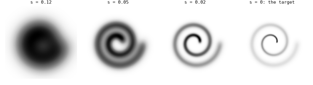
During the stages, the gaussians of a group much smaller than $s$ are merged into one, of the same mass, mean and second moment: a cell then sees a few terms, however many gaussians the group holds. The last stage, at $s=0$, is the mixture itself.

Derivatives

sdot.w2 and sdot.plan are differentiable with respect to positions, sigmas and weights, with JAX or PyTorch. The Gaussian mixture fit finds the gaussians of a point cloud by a gradient descent on $W_2^2$.

Reproducing the pages

They are written by docs/guide/distributions/gaussians_figures.py:

python docs/guide/distributions/gaussians_figures.py                    # all of them
python docs/guide/distributions/gaussians_figures.py spiral widths      # or some of them ( trefoil: long, see the limits )

Limits

• Isotropic gaussians only: one sigma per gaussian. Axis-aligned and general covariances are planned.
• In 3D the solve is slower than in 2D: the Lloyd iterations of the trefoil above take 75 s on an RTX A6000 and 150 s on 24 cores of a Xeon Gold 6258R ( node22 of a cluster, kernels already compiled; the card shared with another process ). The card walks the same tree as the CPU, which gives each cell only the gaussians near it, merged at the width of the continuation, and descends the continuation as adaptively; before them, every cell integrated every gaussian through all 15 stages and the card took about 4.5 min. On the CPU, 46 min became 3.3 min ( a workstation ) when the cells were integrated by their edges rather than by tetrahedra. The 2D spiral takes 5 s.
• No partial transport yet: a gaussian over a polygon inter a disc has no closed form.
• On a CUDA device, a periodicity takes a group of translations ( rotations and symmetries: the CPU ). Under jax.jit, where the centers cannot be read, the copies are those of the images that the diagram walks: tails reaching beyond them are lost.