Images and Splines

An image is a piecewise function on a grid of pixels: a constant on each pixel, or a polynomial. SplineGrid builds a smooth one from values on the pixels, a B-spline written as an image of polynomial pixels.

target = sdot.Image( values )                           # values [ nx, ny ]: a constant per pixel
target = sdot.Image( coeffs, degree = 2 )               # coeffs [ nx, ny, 9 ]: a polynomial per pixel
target = sdot.SplineGrid( values, degree = 3 )          # values [ nx, ny ]: a cubic B-spline ( C2 )

The Mona Lisa as a cubic spline of 80 × 120 values ( its darkness ), quantized by 20000 diracs:

Open in a separate page ↗

The same 12 × 12 values, as constant pixels and as splines of degree 1 and 3 ( left to right ), with the diracs of a Lloyd quantization ( sdot.quantization( target, 1500 ) ):

Open in a separate page ↗

The constant pixels have edges, and the diracs see them. The splines do not, and need no finer image.

Placing the grid

values is indexed as [ x, y, ... ]. By default the image fits in the unit square ( cube... ): its longest side has length 1, and the proportions are kept. To place it elsewhere:

• origin: the corner of the image;
• frame: the edges of the whole image, as rows ( [ d, d ] ), or their lengths for an axis-aligned image ( [ d ] );
• pixel_frame: the edges of one pixel instead;
• knots: the positions of the pixel borders along each axis ( [ d, n + 1 ], in units of pixel_frame ), for pixels of different sizes.

The density is zero outside the image, and the image is the domain of the transport: the cells are cut by its border.

Polynomial pixels

Image( coeffs, degree = p ) takes a polynomial of degree p along each axis on every pixel. It is written in the Bernstein basis of the pixel, in its own coordinates $t\in [0,1{]}^d$:

$$\rho (x)=\sum _{\alpha }{c}_{\alpha }\prod _a{B}_{{\alpha }_a,p}(t_a),B_{i,p}(t)=(\genfrac{}{}{0ex}{}{p}{i})t^i(1-t{)}^{p-i}.$$

coeffs is [ pixels..., ( p + 1 )^d ], the coefficients of a pixel flattened in C order ( the first axis the slowest ). Coefficient $\alpha$ sits at the point $\alpha /p$ of the pixel, and the density follows it without going through it:

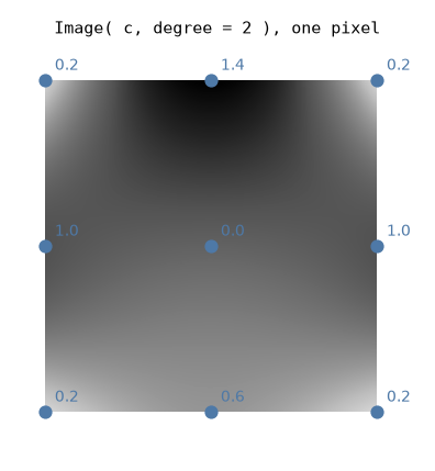
• Non-negative coefficients give a non-negative density.
• The mass of a pixel is its volume times the mean of its coefficients.
• Pixels are independent: the density may jump from one to the next. A spline is continuous because its coefficients agree on the borders.

A density smooth by pieces, with jumps between the pieces, is thus written exactly as long as the jumps follow the borders of the pixels. Here four bands, each with its own wave, alternately dark and light, as constant pixels ( their means ) and as pixels of degree 3, whose coefficients interpolate the function of their band:

Open in a separate page ↗

The constant pixels add steps of their own inside the bands; the polynomial ones keep only the jumps between the bands.

Splines

sdot.SplineGrid( values, degree = 3, frame = None, pixel_frame = None, origin = None, interpolate = False )

The tensor-product B-spline of degree degree ( $C^{degree-1}$ ) whose control coefficients are values, one per pixel, at its center. The grid is placed as for an Image.

• Non-negative values give a non-negative density, and constant values a constant one: the coefficients are extended beyond the border by their edge value.
• interpolate = True: values are samples at the centers of the pixels, and the spline goes through them. Near a sharp edge such a spline dips below zero: it is then refused with a ValueError. A lower degree, or interpolate = False, keeps it non-negative.
• degree = 0 is the image itself.

The result is an Image( degree = degree ): each span of the spline is one polynomial pixel. For an odd degree the spans end at the centers of the pixels, so the image has one more pixel along each axis, half wide at both ends.

In 3D

The same, with values [ nx, ny, nz ]. A cubic spline of 28³ values carried by a gyroid, and 8000 diracs, colored by their depth in the view ( warm in front; c switches it ):

Open in a separate page ↗

What is computed

The cells are integrated exactly, whatever the degree: the masses, the barycenters, the transport cost, and the facets of the Newton system ( a rule exact for polynomials on simplices, Grundmann–Möller ). Everything derives with respect to the coefficients ( or values of a SplineGrid ), the frame and the origin.

The continuation

A target far from uniform needs the width continuation: the solver first transports to a smoothed density, then to sharper and sharper ones ( Iterative( continuation = "auto" ), the default, or "always" ). The stage at width $s$ is the image blurred by a gaussian of width $s$ ( non-negative, with the mass of the image ). It tends to the image as $s\to 0$, jumps included.

On a peaked 64 × 64 target with 2000 diracs, the plain Newton does not converge, and the continuation takes 0.3 s for degree 0, 1 or 3.

Reproducing the pages

They are written by docs/guide/distributions/image_figures.py ( the painting: the public-domain scan of Wikimedia Commons, in data/mona-lisa.png ):

python docs/guide/distributions/image_figures.py                  # all of them
python docs/guide/distributions/image_figures.py mona             # or some of them

Limits

• Polynomial pixels need 2D or 3D. The 1D transport ( a sort ) takes a constant per pixel only.
• The CUDA card integrates constant pixels only; polynomial images are tested on the CPU only.
• Partial transport ( sink_weight ) takes constant pixels only.